How Databases Store Your Tables on Disk

After you complete this article, you will have a solid understanding of:

• How is a table you create in a database stored behind the scenes?
• What are pages and heap files, and how do they work?
• What are indexes and clustered indexes, and how do they provide optimization?
• How do databases work internally?

When you're building a project and set up a database, creating a table with rows and columns feels pretty straightforward. You define the structure, add some data, and it just works. But have you ever stopped to think about what’s actually going on under the hood? How does your computer store all that information behind the scenes?

After all, computers don’t really “know” what a table is, they only deal with 0s and 1s. So how do they take that nicely structured data and translate it into something they can work with?

If you’ve ever created a database and found yourself wondering how rows, columns, and individual cells are really stored in memory, then you’re in the right place. In this article, we will break it all down in a way that’s easy to follow.

Along the way, we’ll also explore some key concepts (Heap file, Index, Clustered Index…) from the world of databases, either you’ll learn something new, or you’ll get a clearer understanding of stuff you might’ve already heard of.

First, let’s start by clearing up some concepts. These concepts are essential to truly understand what’s really happening behind the scenes when it comes to storing your database in a computer’s memory.

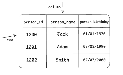
So basically, in a table, we have rows and columns. The photo shown above has rows and columns defined by us.

But in some popular databases, there’s also a column that’s hidden from us. For example, databases like PostgreSQL have a system column called row_id (tuple_id,ctid). So databases create their own internal system to track your table’s rows.

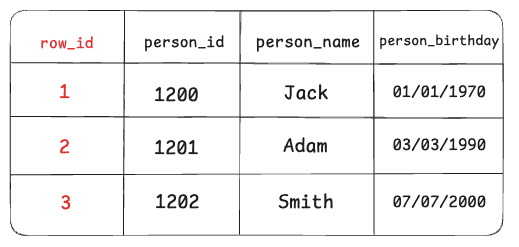
Note: A tuple ID is a pair (block number, tuple index within block) that identifies the physical location of the row within its table. (From postgresql documentation)

But not all databases handle things the same way.

For example, in InnoDB (MySQL's default storage engine);

If the table has a PRIMARY KEY, InnoDB uses the PRIMARY KEY as the row ID.

In this case, the data is physically stored on disk in the order of the PRIMARY KEY (as a clustered index -you will learn what a clustered index in this blog later-). No additional internal row ID is created, the PRIMARY KEY is sufficient to uniquely and physically identify each row.

So if there is primary key: PRIMARY KEY = Internal row ID.

If the table does NOT have a PRIMARY KEY, InnoDB automatically creates a hidden 6-byte row ID (an internal integer column). This hidden column is not visible to the user, but it is assigned to every row. This internal row ID is used to uniquely identify and reference rows internally.

If there is no PRIMARY KEY or even a UNIQUE key, this internal ID becomes essential for performance and referencing.

So If there’s no PRIMARY KEY: InnoDB creates a hidden internal row ID.

This row_id concept is important to know because as we go further, we’ll see actual use cases of these row IDs.

Alright, so now our database has a way to uniquely identify each row, whether through a primary key or a hidden internal ID. That means we’re ready to start thinking about how all this data actually gets stored in memory.

Pages

Okay, now we have a logical table with rows and columns. But how is it actually stored on disk? Obviously, our disk doesn’t store this table as a “table” - it doesn’t even know what a table is.

Depending on the storage model (row vs. column storage), the rows are stored and read in logical pages.

If you don’t know what a storage model is, I’ll briefly interrupt your reading to explain it.

Storage model means that how data is physically stored.

Row Store (Row-based storage)

• This is the most classic and widely used storage model. (Used in systems like MySQL InnoDB, PostgreSQL, etc.)
• In a row store, all the column values for a single row are stored together. Example:

Row 1: [id=1, name="Ali", age=25]
Row 2: [id=2, name="Ayşe", age=30]

Advantage: Very fast for row-based queries (like SELECT * FROM table)

Column Store (Column-based storage)

• Here, data is stored by columns instead of rows. Example (physically stored):

Column id:   [1, 2]
Column name: ["Ali", "Ayşe"]
Column age:  [25, 30]

Advantage: Much faster for analytical queries (like SELECT AVG(age)) because only the needed columns are read.

Examples of column store systems: Amazon Redshift, ClickHouse, Apache Parquet files, Google BigQuery, Apache Cassandra (partially).

Now you know what a storage model means. So let’s get back to pages. What does a logical page actually mean?

A page is basically a fixed-size block of data, either in memory or on disk.

Databases don’t read a single row; instead, they read a page or more in a single I/O, giving us many rows at once. RAM (as the name says, Random Access Memory) allows direct access to any specific memory address, enabling efficient reading of small or individual data blocks. On the other hand, disk storage reads and writes data in fixed-size pages, not individual bytes.

The database allocates a pool of memory, often called buffer pool. Pages read from disk are placed in the buffer pool.

Once a page is loaded into the buffer pool, you don’t just get the specific row you asked for, you also get all the other rows stored on that same page. So depending on how much space each row takes up, you might end up with several useful rows already in memory, basically for free.

This makes reading data much more efficient, especially when doing index range scans. If the rows are small, more of them can fit into a single page. That means each time we read a page from disk, we get more useful data out of it, making every I/O operation more valuable.

The same goes for writes, when a user updates a row, the database finds the page where the row lives, pull the page in the buffer pool and update the row in memory and make a journal entry of the change (often called WAL) persisted to disk. The page can remain in memory so it may receive more writes before it is finally flushed back to disk, minimizing the number of I/Os. Deletes and inserts work the same but implementation may vary.

Note: What is WAL? When a user updates data, the database doesn’t write the change to the data file immediately. Instead, it first records the change in a special log file called the Write-Ahead Log (WAL), also known as the journal. This log is written to disk right away, ensuring the change isn’t lost if the system crashes. Later, the actual data file is updated based on the WAL entry.

Each page usually has a fixed size depending on which database you’re using (for example, 8KB in PostgreSQL, 16KB in MySQL…)

Let’s assume each page holds 4 rows, and we have a table with 1000 rows. That means we will have a total of 250 pages storing our rows.

Page 0 → holds the first 4 rows, Page 1 → holds rows 5-8, and so on…

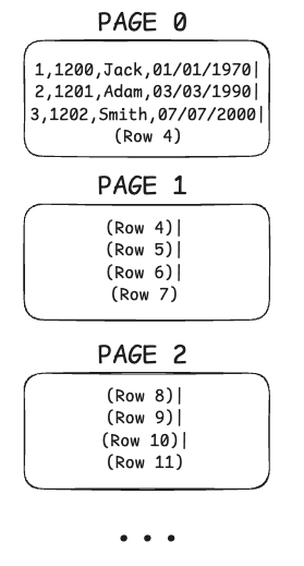(This photo is a simplified example of a pages in row-based storage databases.)

So, in short, a database stores its data in small, fixed-size pieces called pages.

Understanding pages is really important because they are the fundamental factor that can make your queries slow or fast.

Earlier, we said the database doesn’t read a single row; instead, it reads a page or more in a single I/O, giving us many rows at once. But what does I/O really mean in this specific context?

When we say an I/O (Input/Output) operation, we’re talking about any interaction with the disk, whether it’s reading data or writing it. We try to minimize these as much as possible, the fewer I/Os we make, the faster our queries run. An I/O can fetch one page or more, depending on disk partitions and other factors.

Like we said before, an I/O can’t read a single row; it reads a whole page with many rows in it, so basically, we get a lot of rows for free.

But I/O doesn’t always mean going all the way to the disk. Some I/Os interact with the operating system’s cache, which definitely makes your queries faster.

Heap

From now on, we’ll also talk about the “heap” (which usually refers to a heap file). So let’s quickly introduce what that means.

Actually, the heap is exactly what we’ve talked about so far. It’s a data structure where the table’s pages are stored one after another. This is where the actual data lives. Everything in the table is in the heap.

In a heap, pages aren’t stored in any particular order. Data gets placed wherever there’s space, so pages can be scattered and unordered. This means searching through a heap usually means scanning the entire table. (If you use a clustered index, pages are stored in a sorted, organized way based on the index key. You’ll learn what a clustered index is later in this blog.)

So basically,

Heap File → Contains Pages,

Page → Contains Records(rows)

Traversing the heap is an expensive operation since it contains everything. That’s why we need some kind of logic to help us find exactly which page we’re interested in, in other words, which page holds the data we’re looking for. That’s where indexes come in. Indexes help us to tell exactly what part of the heap we need to read, or in other words, which page(s) of the heap to pull.

If we know exactly what page to pull to get what we want, the operation becomes much less expensive, as you can probably guess. But how do we actually do that?

Index

An index is just another data structure - usually a B-Tree - separate from the heap that holds pointers to the heap. So indexes aren’t stored in the heap itself, but in their own structure, pointing to the actual data in the heap.

An index contains parts of the data and is used to quickly search for something. You can create an index on one column or multiple columns.

Indexes tell us EXACTLY which page to fetch from the heap, instead of scanning every page and taking a big performance hit.

But indexes aren’t a magical thing, they’re also stored as pages and require I/O to read their entries. So we need to be careful with indexes. The smaller the index, the more of it can fit in memory, and the faster the search will be.

Now, let’s do a simplified example so you can fully understand what an index really is.

Let’s say we’ve indexed the person_id column in our table. (If you forgot how our table looked, check the first photo.)

So, in the heap section, we have pages, right?

Since we indexed the person_id column, now there’s another data structure that holds the index information, not in the heap, but somewhere else. (The image below isn’t a B-Tree, we don’t store indexes sequentially like in the photo, but it’s meant to help you get the idea. In the real world, indexes are usually stored in B-Trees.)

After indexing person_id, outside the heap file, we have another data structure now;

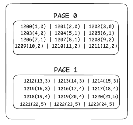
Here, since we indexed the person_id, we store the value of person_id for each row. Along with this value, we also keep information about where to find that row. For example, for employee_id 1200, we know it has a row_id of 1 and lives on page 0.

For employee_id 1204, we know it has a row_id of 5 and is on page 1.

So basically, these numbers mean → employee_id (row_id, which page the row lives on).

The row_id and page info act as the pointers we talked about earlier, directing us to the right spot in the heap section.

Let’s say we want to get the name for person_id 1202. First, we make an I/O request to the index page to find the exact location of that person in the heap. Now that we know the exact location, we make another I/O request to the heap, for example, “give me page 0 and row_id 3.” (We’ll actually pull all the rows in page 0 too, since we can’t read a single row alone, but we only use the data with row_id 3.)

Like I mentioned before, indexes aren’t stored sequentially like in the simple example, they’re stored in a much more efficient structure. So with the right setup, making an I/O request to the index page and finding the correct person_id is very fast, thanks to B-Trees.

Clustered Index

There is also something called a clustered index, which I’ve mentioned earlier in this article. Since it can be really helpful sometimes, I want to explain a bit more about clustered indexes. Like we said before, normally a heap table stores data in no particular order. But if you create a clustered index on a column, the table’s data will be physically organized based on that index.

As you might guess, a table can have only one clustered index because the data can be physically sorted in only one way.

Let's consider a table: Users(id, name, age)

• If this table has no indexes, it is called a heap table. (like we said earlier.)
• If we create a clustered index on the id column:
  • The table is now physically sorted based on the id column.
  • The database stores the data according to this order.
  • This makes queries like WHERE id = 100 much faster.

And in some databases, like InnoDB, every table is actually stored as a clustered index structure as default.

This is because InnoDB physically sorts and stores the data based on the table’s primary key.

If the table has a PRIMARY KEY, InnoDB creates the clustered index on that column, and the data is organized according to that order.

If the table does not have a PRIMARY KEY, InnoDB automatically creates a hidden clustered index, usually based on a unique row ID generated internally in the order the rows were inserted.

So, every table in InnoDB always has a clustered index.

This is actually very important to understand. Let’s say you’re using InnoDB and you have a completely random value like a UUID as the primary key of your table.

Believe it or not, this can seriously hurt your performance. Why? Because since a UUID is completely random, each new row gets inserted somewhere in the middle or a random place in the table. This causes InnoDB to constantly reorganize data, leading to page splits and fragmentation.

As a result, disk and memory accesses increase, and both write and read performance degrade.

So, if you must use UUIDs, it’s better to use them as a non-clustered index, not as the PRIMARY KEY.

For the PRIMARY KEY, using auto-increment integer values is usually better because inserts happen at the end of the table, reducing the need for reorganization.

In InnoDB, other indexes (secondary indexes) do not point directly to the row data, but instead point to the primary key of that row.

In other words:

Secondary index → primary key value → actual row data.

Note: The term "other indexes" refers to the indexes you create using CREATE INDEX or by defining a column as UNIQUE or INDEX.

Example:

CREATE INDEX idx_name ON users(name);

Here, idx_name becomes a secondary index, and InnoDB uses this index to find the primary key value first, then accesses the actual row using that primary key.

But in Postgres, everything is actually a secondary index. Remember, we have row_id (or tuple_id, ctid) in Postgres. All indexes point directly to the row_id which lives in the heap.

So, indexes show row_ids, and row_ids show the exact location of the row.

But there is also an important thing you should know. This might be a bit off-topic for this article, but if you’re a curious and want to research more about database implementations, you can keep reading. After that, you can do your own research on this topic.

ANY update in Postgres will update all the indexes corresponding to that table. Why? Because when you make an update in Postgres, you actually do a DELETE + INSERT. So you create a new row with a different tuple_id. And all the indexes, since they point to that tuple_id, have to know about this new tuple_id, which is why they need to get updated.

Why did I say that when you make an update, you actually do a delete + insert though?

PostgreSQL does not update a table row in place. Rather, it writes a new version of the row (the PostgreSQL term for a row version is “tuple”) and leaves the old row version in place to serve concurrent read requests. VACUUM later removes these “dead tuples”.

If you delete a row and insert a new one, the effect is similar: we have one dead tuple and one new live tuple. This is why people say that “an UPDATE in PostgreSQL is almost the same as a DELETE, followed by an INSERT

Why? Because PostgreSQL uses an MVCC (Multi-Version Concurrency Control) architecture. MVCC allows multiple transactions to read and write data concurrently in a consistent and non-conflicting way by keeping old and new versions of rows. If you’re curious, you can continue researching this topic further. I’m not going into the details here to avoid going too far off the main subject of this article.

I hope after reading this article, you have gained some insight into how databases work internally.